Category Archives: Promise of Data

Uber Data Determine The Best Food Places In New York City

Anyone who lives in the Ditmars neighborhood of Astoria, Queens will speak fondly of El Rey Del Taco, a neighborhood favorite food late night food truck that often has a line down the block. However, it isn’t the only place in the area; in fact, there is another much less popular taco place 50 yards away. What makes El Rey del Taco great (besides the life-changing carne asada) is the location. You can find it on the corner of Ditmars and 31st St where the Q train lets out, perfectly poised to capture party-goers trudging back from Manhattan bars.

Despite how much New Yorkers love their favorite food trucks, the City of New York has set hard limits on the number of them allowed, to curb noise and air pollution from their gas-powered generators. This poses the question: If only a few thousand food trucks can legally operate at any given time, what is the best real estate. How can they best optimize their locations to maximize sales? While spots like the major subway stops are no-brainers, most of these sites have already been claimed. On top of that, the city plans to increase the number of permits substantially over the next several years, and these carts will need to find new spots.

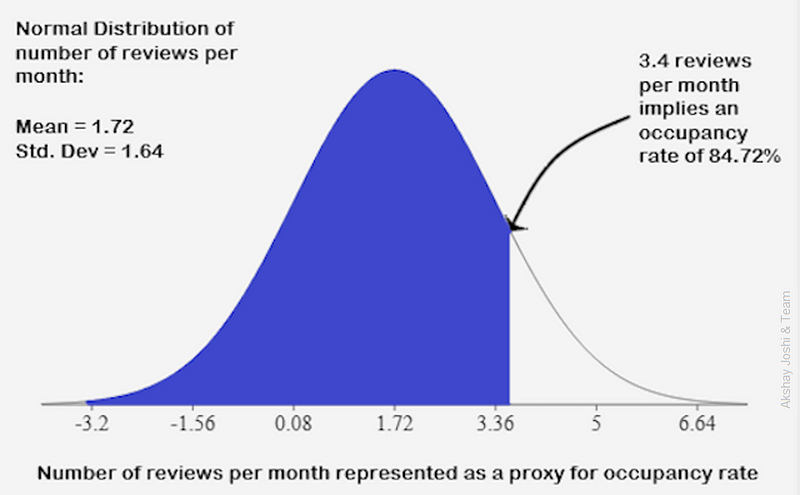
Can location data from mobile devices provide a reasonable proxy for the concentrated volume of potential customers? Using a public Uber dataset, we looked at all the pickup and drop off points that occurred over a 3-month time window within Manhattan. Obviously, this data set doesn’t capture all people on the move (pedestrians, Yellow cab riders, bikes, etc.,) but it roughly reflects high traffic locations in NY and thus can be a primer for food truck locations.

Best Food Truck Locations in NYC can be determined by data.


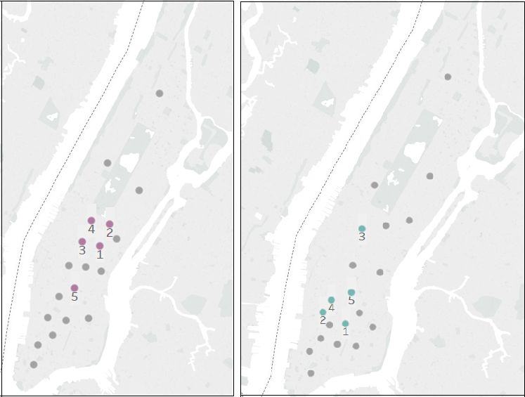
The data set comes in the form of spatial coordinates. A heat-map of all pickups will show the expected: Manhattan is a very busy place. To yield more exact results, we used a K-means clustering algorithm to pinpoint cluster centers within the traffic data. The underlying idea is that a cluster center generated from this dataset would generate spots on the map that minimize distances between pickup points, indicating locations with ideal points to set up food carts to access the highest number of customers. Once we assigned each pick-up data point to a cluster (Figure 1), we ranked the clusters based on pickup volume (Figure 2).

Figure 1: Pickups colored by cluster assignment


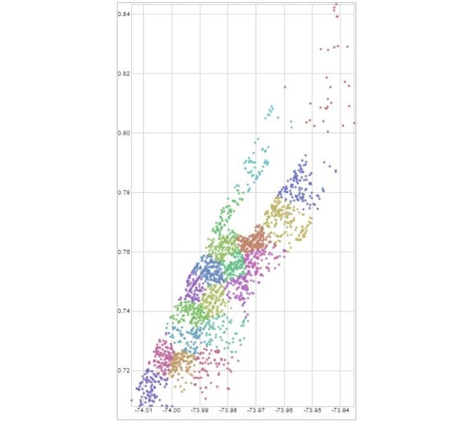
As you can see from Figure 1, there are significant differences between the cluster centers and the top-ranked points at different times. While the main centers of pickups are around Greenwich Village and Lower Manhattan on Thursday evenings, late on Saturday night the traffic centers around Midtown. Especially for smaller, fully mobile carts (think ice cream trucks with a driver or Italian ice carts), this kind of information could help tell operators where to go to take advantage of Uber customers. Nevertheless, using a k-means has shortcomings. The distance is Euclidean and not along the actual roads, so it might be that a center seems close but in reality, it is not. Moreover, this assumes that Uber users are good food truck customers.

Figure 2: Thursday evening vs. Saturday late night top ranked cluster centers.


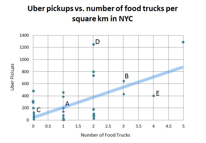
To test the hypothesis that there is a relationship between Uber pickups and food truck locations, we triangulated our Uber data with food truck location data scraped from Yelp. We then divided the city into a grid and determined how many total pickups and food trucks occurred in a given square kilometer. In each grid square, we calculated a ratio of Uber pickups to the number of food carts.

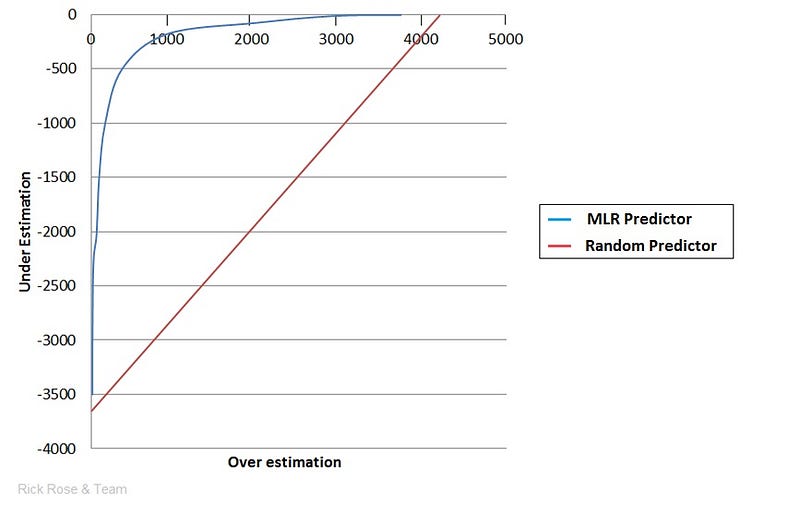
While we found that there was a positive trend between the number of pickups and the number of trucks in a given area, a multiple linear regression revealed that the relationship was not significant; in other words, while Uber pickups increase in a given area so do the number of food trucks (see the upward trend in Figure 4), but you can’t predict the number of food trucks by the number of Uber pickups with statistical significance. Thus, based on this model alone we can’t confirm that Uber pickups create a good signal for food cart locations. While Yelp was the largest and most complete data set on food truck locations that we could find, there may be food trucks that do not appear on the site. This could explain some of the lack of significant correlation. Regulations about where food trucks can operate might also influence the results. On the Uber side, there are other transportation methods that cannibalize Uber traffic like subway stops, which is another variable not captured in our model.

Figure 4: Number of Uber pickups vs. number of food trucks by square kilometer in Manhattan; each individual point represents a specific square kilometer space, located on the chart based on the number of Uber pickups and number of food trucks that fall within that area in a defined time frame.


This lack of correlation could have a few interpretations: there are unexplained variables in this data (other forms of transportation skew the results), our initial assumption that Uber users are good food truck customers is off, or that food truck locations are not optimized to meet this source of demand.

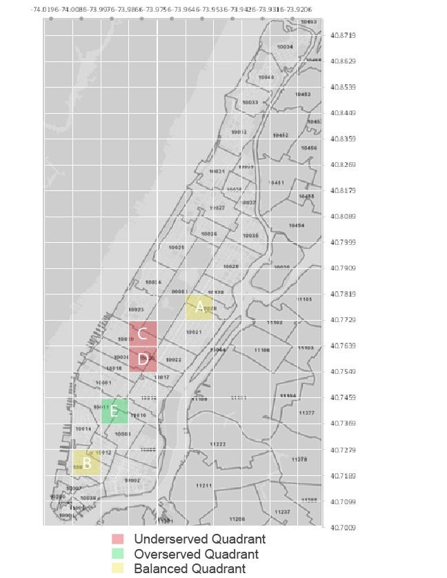
If we maintain the assumption that Uber users are good food truck customers, we can use our trend analysis to determine whether certain areas are under- or over-served by food carts. For example, while a spot known to have good foot traffic might have several food trucks, is the ratio of food trucks to the number of pickups high or low? This could give us a sense of how well balanced the supply of food trucks is given the demand generated by Uber customers. Then, potential food truck operators could use this information to spot areas where supply might not meet the potential demand.

As you can see from Figure 4, there are areas where the trendline predicts roughly how many food trucks can be expected based on the number of Uber pickups (points A and B). However, there are points where there are an average amount of Uber traffic but zero food carts ©, above average Uber traffic with an average number of food trucks (D), and points with below average UBER traffic and a well above average number of food trucks (E). These disparities roughly define areas that may have an opportunity to better optimize food truck locations by either adding more carts to the system in underserved areas that may not meet demand and moving trucks away from overserved areas that may be over-saturated (see Figure 5).

Figure 5: Under-/Over-served quadrants from Figure 4 mapped


With the proliferation of user-based apps that contain valuable insights around how individuals interact and move around, business decisions can increasingly be driven with data. This analysis provides one perspective on how app data from sources like UBER can be used to inform seemingly unrelated businesses, showing the potential to incorporate external data sources in addition to internal ones. However, even combined data doesn’t always paint a complete picture. Sometimes a food truck is just so good it doesn’t matter where it is (or how bad the service is); it’ll always have a line.

This article was co-authored by Katherine Leonetti, who recently finished her MBA with a concentration in Sustainable Global Enterprise at the Cornell Johnson School of Management. She will be working for Citibank’s Technology and Operations division and located in Mexico City, where she hopes the carne asada will meet her high expectations. The original project was a collaboration with Katherine, Swapnil Gugani, Tianyi (Teenie) Tang, and Wu (Will) Peng, developed for the Designing Digital Data Products course at Cornell that Lutz Finger is teaching.

Lutz Finger is Data Scientist in Residence at Cornell. He is the author of the book “Ask, Measure, Learn”. At Snap & LinkedIn he has built Data Science teams.

This Article was originally published on my Forbes blog.

How A Small Restaurant Can Use Its Data

How can small businesses leverage point of sale data to make informed decisions? Big Data sounds often like Big Business, but the power of data is available even to small businesses without extensive resources. Point of sale data coupled with Excel and basic statistical knowledge can be leveraged to drive informed decisions and make businesses data driven.

A group of Cornell University graduate students from my class “Designing Data Products” set out to help an iconic yet small family owned restaurant on the Jersey Shore to leverage its point of sale data, to make informed decisions around inventory management.

The Circus Drive-In Restaurant serves approximately 100,000 customers looking to explore the beaches in the summer. Due to its close proximity to the shore, the primary driver of customer numbers is the weather. “The unpredictability of the weather makes inventory management extremely difficult,” says Richard Rose, co-owner, and general manager. The restaurant’s top sellers are the fresh, made-to-order burgers. “We do not use frozen meat for our burgers”, says Rose.

The Circus Drive-In is a fast food hamburger drive-in restaurant that opened in 1954.

This approach makes the logistics even more challenging. If the restaurant overstocks its meats and has leftover inventory, the meat is not used and has to be thrown away, leading to spoilage costs. On the other hand, understocking of meat will lead to dissatisfied customers and lost revenue, both of which are detrimental to a seasonal business.

The restaurant manager manually tracks inventory usage on paper. The forecasting process is a combination of channeling the manager’s inner meteorologist, economist, and restaurateur. It is a gut feeling based on invaluable experience which helped get the business to where it is today. However, in the world of data ‘gut’ and ‘experience’ can be augmented by predictive data analytics.

The Cornell team created a model to predict demand for hamburgers. The model utilized point of sale data from 2015 and 2016, along with weather, seasonality, and holidays. Often getting data is a challenge. However historical weather data is particularly easy to obtain from web archives. The statistically relevant variables were maximum daytime temperature, average humidity, and the likelihood of thunderstorms. The holiday data was obtained from the website OfficeHolidays. Once the data had been collected, as usual, most of the work involved getting the data into the right format. The team had to spend some time to transform the data to make it usable, for example, converting holidays into Boolean dummy variables for the model.

Approaches to forecasting can range from simple moving averages via autoregressive integrated moving average (ARIMA) to probabilistic forecasting and ensemble forecasting. Often simpler algorithms and easy tools are powerful enough to get a quick win. In this case, the team used Excel with a XLMiner plugin. Not fancy but sufficient!

Running a regression is a two-step process. First, a partition process creates randomly selected training and test datasets from the original dataset. Second, a build and test process produces the regression model and performance metrics. The graph below shows how effective the model is by comparing under-estimation vs. over-estimation per season. To explain the graph, there are two curves, the Random Predictor and MLR Predictor, which when compared express the benefits gained by using the model. To ensure that the restaurant has sufficient hamburger inventory at all times, the restaurant will need to massively overstock, representing over 4,200 patties wasted. This is shown by the intersection of the Random Predictor (red curve) with the horizontal axis. If the restaurant is willing to run out of patties on occasion and experience accumulated lost sales of let’s say 500 hamburgers, it still would need to stock 3,800 patties more than needed. Using our model (blue MLR curve) under the same circumstances, the amount of waste can be reduced to 700 patties, saving 3,100 hamburger from being disposed of.

Under vs. Over-Estimation — Using A Random Guess vs. The Model

This frees up working capital, improves the baseline return and prevents food spoilage as well as freeing up the manager’s time to focus on the restaurant’s operations instead of gut-feel forecasting.

In the area of big data, we often forget that the success of data is often based on the actual questions. Small business owners know their businesses best, and know what to ask the data: in this case, “how can I stock hamburger meat up correctly.”

Small businesses often have good control of their data. If the wealth of information from their own point of sales system is not sufficient, one can easily merge publicly available data, as the team did with weather and holiday information. Often no complex tools are needed to make data work. With that, let’s get down to the beach of the Jersey Shore and enjoy a burger — hopefully data driven!

This article was co-authored by Jean Maldonado, Jiangjie Man, Rick Rose, and Riya Sarkar. Jean Maldonado and Jiangjie Man recently finished their Masters degrees in Information Science from Cornell University, and Rick Rose and Riya Sakar will be completing their Masters in Business Administration at the Johnson Graduate School of Management at Cornell University in 2018. All of them will focus their career in a data-heavy environment. Jean Maldonado is a Data Management and Analytics Consultant at Eccella Corporation, Jiangjie Man is pursuing a career in software engineering, Rick Rose is pursuing a career in brand management, and Riya Sakar is pursuing a career in technology strategy. Please reach out on LinkedIn to them if you would like more information about this project that was developed for the Designing Digital Data Products course at Cornell, taught by Lutz Finger.

Lutz Finger is Data Scientist in Residence at Cornell. He is the author of the book “Ask, Measure, Learn”. At Snap & LinkedIn he has built Data Science teams.

This article was originally published on my Forbes Blog.

Should You Airbnb Or Sell Your Property — Big Data Helps

Data-driven decision making is a practice in many commercial industries now. But especially the real estate industry is using data. Companies like Zillow or Redfin provide estimates of a given house in a given neighborhood for renters and buyers alike using historical data. But, there is a third option besides ‘selling’ or ‘subletting’ a house. You could rent it out via Airbnb. There’s no tool that predicts your income from this third option. Let’s build one.

Students of my class at Cornell University created a small neat tool to help you with that decision. Real Estate Advisor lets you enter the address of your spare property (in L.A. only for now) that helps you evaluate the two options on hand — AirBnB and Sell. Check out this video on how data could help you make a decision quickly:

Let’s look at what happens in the backend when you hit the “Predict” button. Real Estate Advisor predicts the potential selling price of your house today and compares it to the potential revenue that you could make using prices as seen on AirBnB for similar houses. Like house prices, the potential AirBnB income depends mostly on the number of rooms. Thus, much like a hotel the more rooms there are, the higher the income. Airbnb, however, has a higher rate of seasonality. (Note: The Airbnb prices in the US see a seasonality which we did not include into our discussion here.)

Below, the team of Cornell University students shows how they predict both the property price and the expected perpetual income via Airbnb.

 Using Big Data to decide whether to sell or rent a property

How to calculate the selling price of your property?

Predicting housing data is a typical exercise that many data scientists do. To predict the property price, we need the real estate data. And in this era, there’s no dearth for datasets (for instance, here are many datasets at Kaggle). But data is like vegetables — it perishes easily. Thus, for Real Estate Advisor to work, recent data is needed. Websites like Redfin, Zillow or Trulia can be rather easily scraped to obtain the required data such as the size of the house (in sq.ft), property type, number of beds and baths, lot size (in sq.ft) and, property age. Additionally, we added the quality of the school districts into our model. The proximity to the top schools was calculated by computing the minimum Haversine distance between the schools and the property on sale. The distance to the closest school was then used as a variable.

Using a multiple linear regression model and the student t-test, we selected the variables that passed the test of significance. The R2 of our model was 0.39, showing that there is room for improvement. Also, while comparing our predictions to those on Zillow and others, we can see that we are missing variables and maybe, even need to consider nonlinear models in further iterations.

How to calculate the perpetual AirBnB income of your property?

To create a level playing field for both the sell option and the let out option on Airbnb, the income from Airbnb is assumed to be a perpetuity with a present value.

InsideAirbnb offers great insights for all the regions via a public dataset (insideairbnb.com) that allows us to calculate the assumed price at a given location. In real estate, location plays an important role. We found k-nearest neighbors (k-NN) algorithm the best to capture the significance location has on the rent your property commands. Essentially, if your house is close to houses that are expensive on Airbnb, it’s likely that your house will command a higher rent.

Using k=5, we calculate the average income per guest for each of the 5 nearest listings and arrive at what would be the income per guest from your property and for simplicity, we assume that two guests stay in a room. Then, based on the number of rooms your property has, we calculate the weighted average daily income from your property on Airbnb. The properties closest to yours will have a higher significance. To capture this, the weights used are the inverse of the Haversine distance between each of the nearest Airbnb listings and your property.

Nearest Neighbors used to define the value

Arriving at the daily income from your property on Airbnb is only half the battle. We need to also predict the annual occupancy rate of your property to compute the total annual income from your property on Airbnb. Annual occupancy rates vary by location — while everyone wants to get the nice chalet in the snow in the mountains for Christmas, the demand for the same property will be lesser during the rainy spring season. Occupancy rates are neither publicly available nor easily obtainable. As a proxy, we used the average and standard deviation of the number of reviews per month for all the Airbnb listings and used it as a normal distribution function to calculate the annual occupancy rate. The weighted average of the number of reviews per month of the 5 nearest Airbnb listings is used to predict the annual occupancy rate of your property.

Reviews per month represent the occupancy rate

Once we have the annual occupancy rate, we calculate the total annual income from your property on Airbnb. We treat this income as a growing perpetuity and compute the present value of this perpetuity using your desired return on investment (ROI) and annual growth rate of the income (Inflation) with the formula: Annual Income/(ROI-Inflation). The present value of this perpetual income from Airbnb is compared with the predicted selling price to arrive at a decision to either sell or let out your spare property on Airbnb. If you decide to let out the property on Airbnb, the tool suggests a target annual occupancy rate you need to maintain to remain profitable. The annual occupancy rate of your property on Airbnb is paramount. If you’re able to maintain an occupancy rate of 60–70% on your property, Airbnb would almost always be the most profitable option.

How can you improve the tool?

There is certainly room to improve the tool, both qualitatively and quantitatively. The model does not factor in the fact that Airbnb demands time and effort to maintain your property, while property sale is a one-time transaction. Also, the tool doesn’t take into account other qualitative factors such as the importance of liquidating assets, or the importance of a steady annual income, for property owners.

The predictive accuracy of the tool can be significantly improved with data. We need to consider additional variables such as the number of parking lots, the floor an apartment is on, the presence of a swimming pool etc., to predict the selling price of a property. Similarly, the annual AirBnB income is influenced by other factors such as the annual maintenance costs, proximity to tourist attractions etc.

However, with relatively little effort, we were able to create a tool to help you with the age-old Sell vs. Rent discussion. The availability of data enables everyone to make more informed decisions.

This article was co-authored by Akshay Joshi, Chawisara Uswachoke, and Lihong Lao, who are students at Cornell University. This project was done as part of the Designing Data Products course at Cornell University that Lutz is teaching. Akshay is currently an MBA student at the Cornell SC Johnson College of Business, and will graduate in May 2018. Chawisara is a recent graduate who majored in Information Science, and is looking for data-driven job opportunities. Lihong is a Ph.D. student in Materials Science & Engineering, and will graduate in 2018 as well. Please reach out to them directly via LinkedIn if you would like them to join your team.

UPDATE — Oct 19th — 9:41pm

The dataset used is not offered by Airbnb but by Inside Airbnb an organization founded by Murray Cox. Inside Airbnb is independent of Airbnb. The data from Inside Airbnb is offered under the Creative Commons CC0 1.0 Universal (CC0 1.0) “Public Domain Dedication” license. Additionally, Murray commented that the model has an oversimplification which is the assumption that all rooms in a house can be rented out. There are housing and zoning regulations that affect Airbnb rentals and would not allow the house to be rented out in full.

Lutz Finger is Data Scientist in Residence at Cornell. He is the author of the book “Ask, Measure, Learn”. At Snap & LinkedIn he has built Data Science teams.

This article was originally published on my Forbes Blog.

Binladen Map

Knowing Osama’s Whereabouts

 In April 2011, the United States Special Forces descended on Osama bin Laden, leader of the terrorist group al-Qaida’s, hideout. The ensuing raid killed bin Laden after over a decade of living in hiding and directing attacks through his followers. So who knew where he was located?

The answer may surprise you:

We ALL did.

According to Kalev Leetaru, a researcher at the University of Illinois at Urbana-Champaign, an analysis of public news articles about bin Laden pinpointed his location within 200 kilometers in diameter. In a very real sense, one of the world’s most secretive hiding places may have ultimately revealed itself from the mosaic of individual data points. Each journalist had an opinion about the location, and all opinions together formed a true answer. The catch here: no survey was conducted, and no journalist was actually asked where they thought Osama was hiding. They revealed their opinions on bin Laden’s whereabouts through their articles. This is the power of public and unstructured data.

_55264770_binladenmap

Most likely, the US forces did not rely on crowdsourced wisdom like this. We know today that US governement agencies like the NSA are tapping into all kinds of different data sources, from spying on the phones of top-level politicians to tapping into everyone’s communications through email providers. However, the principle is the same: actionable intelligence was derived from the aggregation of individual, and in this case, seemingly random, data points.

Herein lies the promise of what we call big data. It has become one of the trendiest digital buzzwords of the new millenium. It involves gathering business intelligence from the heretofore forbidden territory of data sets that are too large to curate or maintain as databases, often encompassing terabytes or even petabytes of information.

The text is part of the INTRO chapter from Ask – Measure – Learn.